Introduction
Why cloud-native raster analytics?
Traditional raster workflows often assume:
- Data lives on a local disk or a mounted drive.
- Full scenes or tiles are downloaded before analysis.
- Processing is limited by RAM and single-machine CPU.
Cloud-native workflows invert this:
- Discovery happens via catalogs (STAC) over the web.
- Data stays in the cloud; only the required windows or bands are streamed (e.g. via COGs).
- Compute can be chunked and parallelized (Dask) so that large rasters never need to be fully loaded.
The same code can then run on a laptop or a cluster, including continental or global multi-temporal rasters.
Workshop overview
This workshop covers a cloud-native raster pipeline in Python: find data, stream it, model it as a cube, and scale the compute.
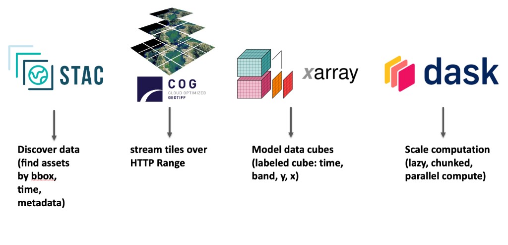
| Topic | Tool | Lesson |
|---|---|---|
| Search satellite rasters by place, time, and metadata (e.g. cloud cover) | STAC | 1. STAC & COG |
| Stream only the required tiles over HTTP — no full-scene download | COG | 1. STAC & COG |
Model rasters as a labeled cube (time, band, y, x) and select by name |
xarray | 2. Data cube |
| Attach CRS, clip, and reproject inside xarray | rioxarray | 3. rioxarray |
| Run chunked, lazy, parallel analytics that fit in memory | Dask | 4. Dask |
| Assemble one vegetation-monitoring application from search to maps | all of the above | 5. Application |
Tooling overview
| Layer | Tool | Purpose |
|---|---|---|
| Discovery | STAC (pystac-client) | Search catalogs by bbox, time, and metadata |
| Storage / transfer | Cloud-Optimized GeoTIFF | HTTP range requests; read windows without full download |
| Data model | xarray | Labeled N-dimensional arrays (the “cube”) |
| Geospatial | rioxarray | CRS, bounds, and GeoTIFF/COG I/O in xarray |
| Compute | Dask | Lazy, chunked, parallel execution |